

This new investigation into the impact of California‘s infamous Proposition 13 (to which many researchers trace the beginning of the Golden State’s decline and fiscal crises) essentially suggests that not only has prop 13 inhibited the turnover stock, it has also inhibited the fixing-up of older properties.
But there are many other implications:
- Less turnover equals less revenues for appraisers, lenders, brokers, moving companies, less capital improvements to buildings
- Neighborhoods will have suboptimal housing that is left in poor condition for fears of re-appraisals
- People will live in less than optimal matches in terms of the right sized home for themselves
- Supply will be reduced in neighborhoods, especially of olde3r homes and this artificially raises prices significantly for everyone is such areas
- Over time this problem will get worse as the present value of savings becomes so large that even fewer people will move or sell homes
In other words, Proposition 13 is a magic formula for the devitalization of residential neighborhoods. While many would like to see Prop 13 overturned entirely, it need not be overturned in order to eliminate its devitalizing effect on neighborhoods. It simply needs to be altered by limiting it to one generation.
Currently, it is inter-generational: it can be passed on. If that “heir benefit” were eliminated, it would achieve its purposes of not forcing people out of their homes, but the problem of not being able to sell would phase out when the existing owners passed away. California can keep Prop 13, but limiting it to one generation would mitigate some of the problems forecasted in this research.
This paper, “The Impact of Prop 13 on Effective Tax Rates, Turnover and Home Prices“, will be officially published later in 2016 by The Journal Of Housing Research. It appears first here in REVITALIZATION courtesy of author Norman G. Miller, Ph.D., as well as his co-author, Michael A. Sklarz CEO of Collateral Analytics, Inc., and Hoyt Fellow.
Dr. Miller is a Professor and the Ernest W. Hahn Chair of Real Estate Finance at the Burnham-Moores Center for Real Estate of the University of San Diego, in San Diego, California. You can email him at nmiller@sandiego.edu.
See Dr. Miller’s Sustainable Real Estate Scoop account.
FULL PAPER APPEARS BELOW
<h3>The Impact of Prop 13 on Effective Tax Rates, Turnover and Home Prices</h3>
By Norman G. Miller* and Michael A. Sklarz**
Forthcoming in the Journal Of Housing Research
Abstract: Prop 13 has been around since 1978 and limits annual property tax increases to no more than 2% per year while property values have increased by several times this amount resulting in much lower property taxes on long held properties. Over time, as property tax burdens are restricted to a fraction of neighbor properties owners are dis-incentivized from selling. Florida has a similar Prop 13 policy but it is 50% higher at 3% per year in a state with historically less appreciation. Other states are contemplating this policy as a way to not push homeowners out of their homes. The question addressed here is not one of equity, but rather how much does the reduction in supply of housing affect turnover and prices. We also examine actual property taxes paid which suggest a large portion of the households are substantially benefitting from this policy. Further, we address how much does the lower property tax burden equals on a present value basis as a percent of the total current home value. The answer is shockingly high.
*University of San Diego, Burnham-Moores Center for Real Estate; Collateral Analytics, and Hoyt Faculty. Contact: nmiller@sandiego.edu
**Collateral Analytics, Inc., CEO and Hoyt Fellow. Contact: msklarz@collateralanalytics.com
A Note on the Impact of Prop 13 on Effective Tax Rates, Turnover and Home Prices
Introduction:
Several US states have considered or are considering property tax increase limitations similar to those described below in California, known as “Prop 13”. New Jersey has the highest effective rate at 2.38% of property value, followed closely by Illinois (2.32%), New Hampshire (2.15%), and Connecticut (1.98%). On the other end of the spectrum, Hawaii has the lowest effective rate at 0.28%, followed closely by Alabama (0.43%), Louisiana (0.51%), and Delaware (0.55%). Texas, Michigan, Florida and other states have considered property tax increase limits that are intended to help prevent elderly and lower income households from losing their homes to unaffordable property taxes. In this regard, California has now had Prop 13 long enough to examine its impact on the housing market, which is the purpose of this study. Prior to other states implementing these rules so favored by the aging population, politicians should carefully examine and understand the longer term implications.
Prop 13 has been in effect since 1978. This legislation limits increases in property taxes to no more than 2% per year. It also requires effective property taxes, defined as the total paid per year divided by the value, to be no more than 1% of property market value, although with special assessments the total effective property tax rates range from about 1.02% to 1.21% for homes with full assessments in San Diego County, the area studied here. Because of the ability to pass on the benefits of Prop 13 to the next generation, the longer Prop 13 survives the greater will be the disparity between what the earliest beneficiaries pay in property taxes each year compared to the newest open market home purchasers.
Whether or not you agree with Prop 13 it is interesting to stop and pause and ask just how Prop 13 has affected real estate markets and what people actually pay as of late 2014? We took all the homes in San Diego County and appraised (valued) them using an automated valuation model (AVM) from Collateral Analytics, known to be one of the most accurate in the country. Then we divided this value estimate into the annual property taxes actually paid to derive the effective property tax rate. Last, we grouped homes by neighborhoods with around 10 to 15 neighborhoods per zip code. Here is what we found.
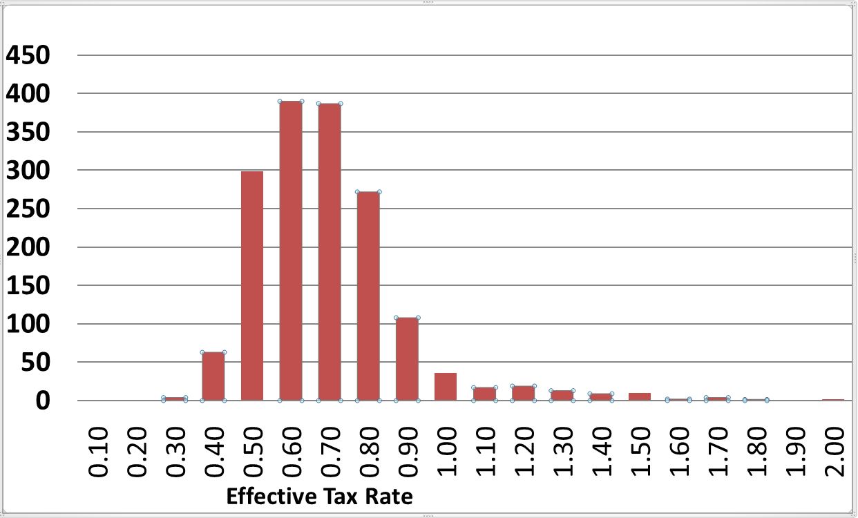
- The average effective property tax rate in San Diego County is 64.36% of the 1% to 1.2% target full assessment rate (i.e. market value). See Exhibit 1 below where 1.0 on the horizontal axis is a 1% property tax rate. This is likely indicative of other coastal cities in California.
- 4.6% of neighborhoods pay more than an average 1% effective property tax rate, presumably because property values have fallen and lower re-assessments have not kicked in yet.
- 22.4% of all households pay less than 50% of the 1% effective property tax with some households paying just a fraction of that.
In neighborhoods with an effective property tax rate less than 50% of the 1% effective rate the turnover of housing is around a third of that for fully taxed neighborhoods. See Exhibit 2 below. Household tenure also increases dramatically.
Exhibit 1: San Diego 1635 Defined Neighborhoods Frequency by Effective Property Tax Rate
Neighborhoods with lower than average effective property tax rates also show a lower turnover rate. We calculated the long term turnover rates from 2005 through 2014. If there were 100 homes in a neighborhood and 100 homes had sold, including repeats, then we classified that as 100% turnover and so forth. So 100% a turnover rate suggests about 10% of the market turns over on average each year. The average turnover rates shown here in Exhibit 2 are much lower than that closer to 3.3% per year over this time period and slightly below national averages. What is clear in Exhibit 2 is that the lower the effective property tax rate the lower is the average neighborhood turnover. The correlation between effective property tax rates and turnover is -.1266%.
Exhibit 2: Turnover Rate of Homes (Percent of Total Inventory Sold Between 2005 and mid-2014) Versus Effective Property Tax Rate

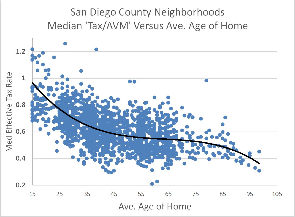
In Exhibit 3 below, we show the one variable we can observe which is highly correlated at -.6024 with lower effective property taxes is the age of homes. Older homes seem to have lower turnover rates and lower property taxes. While we do not have the average length of tenure for owners in each neighborhood, this seems to be a reasonable proxy.
Exhibit 3: Effective Property Taxes by Average Age of Home
Possible Impact of Prop 13 on Home Prices and Prior Literature
Over time the disparity between households paying full property tax assessments and a fraction of the full assessment will grow. The average effective rate in San Diego County and perhaps indicative of the rest of California’s coastal cities is 64% of fully assessed rate. This will continue to drop over time as new beneficiaries continue to hold onto homes rather than sell them to new owners that are subject to full assessment. The present value of saving thousands of dollars in annual property taxes not only discourages external improvements and encourages secret internal capital improvements, so as not to trigger a new assessment, but also results in these homes being much more valuable to the occupants.
While everyone knows about the inequities between neighbors in California paying vastly different property tax rates, an illustration may help to illustrate the size of the benefits and redistribution. In Coronado, full assessment is 1.0478% of market value. One home was pulled at random from this lower than average tax neighborhood pays far less than the average rate. The address is a real property with a faux number and street with actual information as described below:
1000 Lucky Tax Payer Blvd, Coronado, CA. 92118: Built in 1917 this 4 bedroom, 5 bath house is 3524 square feet in size and using an automated estimate of value from Collateral Analytics is worth $2,059,393 as of August, 2014. The property taxes in 2014 were actually $2175 per year. Full assessment taxation would be $21,578 per year some ten times the actual taxes paid. The difference is -$19,403 per year. If we were to use the average rate paid in San Diego County of .64% the difference would still be -$11,005 per year.
What is the present value of the below market taxation to the owner occupant?
Since this return is low risk like treasury bonds, the discount rate should be close to the risk free rate. One might argue the term over which to discount the savings, but is too soon to know and certainly the ability to pass on this tax savings to future generations suggests that many homeowners will keep the below tax situation as long as possible. Think of what they give up if they don’t. Using a generously high 30 year Treasury bond rate of approximately 3.3% we get the following results:
30 Year Present Value of Saving $19,403 per year at a 3.3% discount rate = $365,974
30 Year Present Value of Saving $11,005 per year at a 3.3% discount rate = $207,573
These figures are approximately 10% to 18% of the value of the home.
These present value benefits are implicitly if not explicitly known. What is not as well-known are the price effects of lower turnover and less supply coming on the market in relatively low property tax burden neighborhoods.
The question is whether this lack of supply, as evidenced by the lower turnover rate in Exhibit 2, translates into higher prices based on reduced supply in such neighborhoods. Theory suggests it does.
Ken Rosen in a 1982 study suggested a one-time boost in property values based on the capitalized value of the property tax savings possible in the future, not unlike the calculation above. This study based on the Northern California real estate market found that every one dollar in property tax reduction led to a seven dollar increase in a home’s purchase price. This finding indicated Proposition 13 provided a one-time boost in value, captured by those who owned property at the time it took effect. The author notes that this study, conducted while the state was still able to backfill local revenues, did not capture housing price changes that would result from deteriorating public services. It is not clear that the mobility lock-in effect had been taken into account yet but the benefits suggested were well below those in the above example for the present value to the homeowner. Granted interest rates were much higher in 1982 and that alone could explain the difference.
In a 2004 study by Ferreira called “You can take it with You: Transferability of Proposition 13 Tax Benefits, Residential Mobility, and Willingness to Pay for Housing Amenities” the conclusion was that there was a significant impact on household mobility. Wasi and White (2005) concluded that Prop 13 creates a “lock-in” effect and that the average tenure in California since Prop 13 has been increasing, but that rent controls may explain some of the lock-in impact.
In a more recent study (2014) by Imrohoroğlu, A., Matoba, K., & Tüzel, S. they use theoretical models and simulations to estimate an 18% increase in housing prices and a 17% decrease in the probability of moving, but note that reality suggests a life cycle hypothesis whereby the longer someone is in a home the less the probability of moving.
The lock-in effect described by other studies and the reduction in supply as a result of lower turnover should only increase over time. One can imagine the great-great-great-grandchild of an owner of a property on Coronado paying a small fraction of what the newest neighbors pay will find it almost inconceivable that they could sell such a property. This market distortion is akin to a long term tenant in a rent controlled unit in New York City where the tenant does not have to give up the artificial constraint on rent even when they die. The average effective property tax rate in San Diego County will continue to decline if these trends continue as new beneficiaries continue to hold onto homes rather than sell them.
<h4>Impact on Residential Turnover of Lower Effective Tax Rates</h4>
As of 2014 it is clear that turnover is affected by lower property tax rates. Not only do lower tax rates reduce the supply of housing placed for sale on the market but they also make household less mobile, as suggested by prior studies. The most famous study on the benefits of mobility is probably one by Charles Tiebout (1956). Tiebout’s key insight was that when local governments provide goods to citizens who can move among distinct communities and when citizens are faced with an array of communities that offer different types or levels of public goods and services and different property tax burdens, then each citizen will choose the community that best satisfies his or her own particular demands. Individuals effectively reveal their preferences by “voting with their feet.” Prop 13 effectively reduces the ability of households to vote with their feet and also reduces incentives to make significant capital improvements to homes.
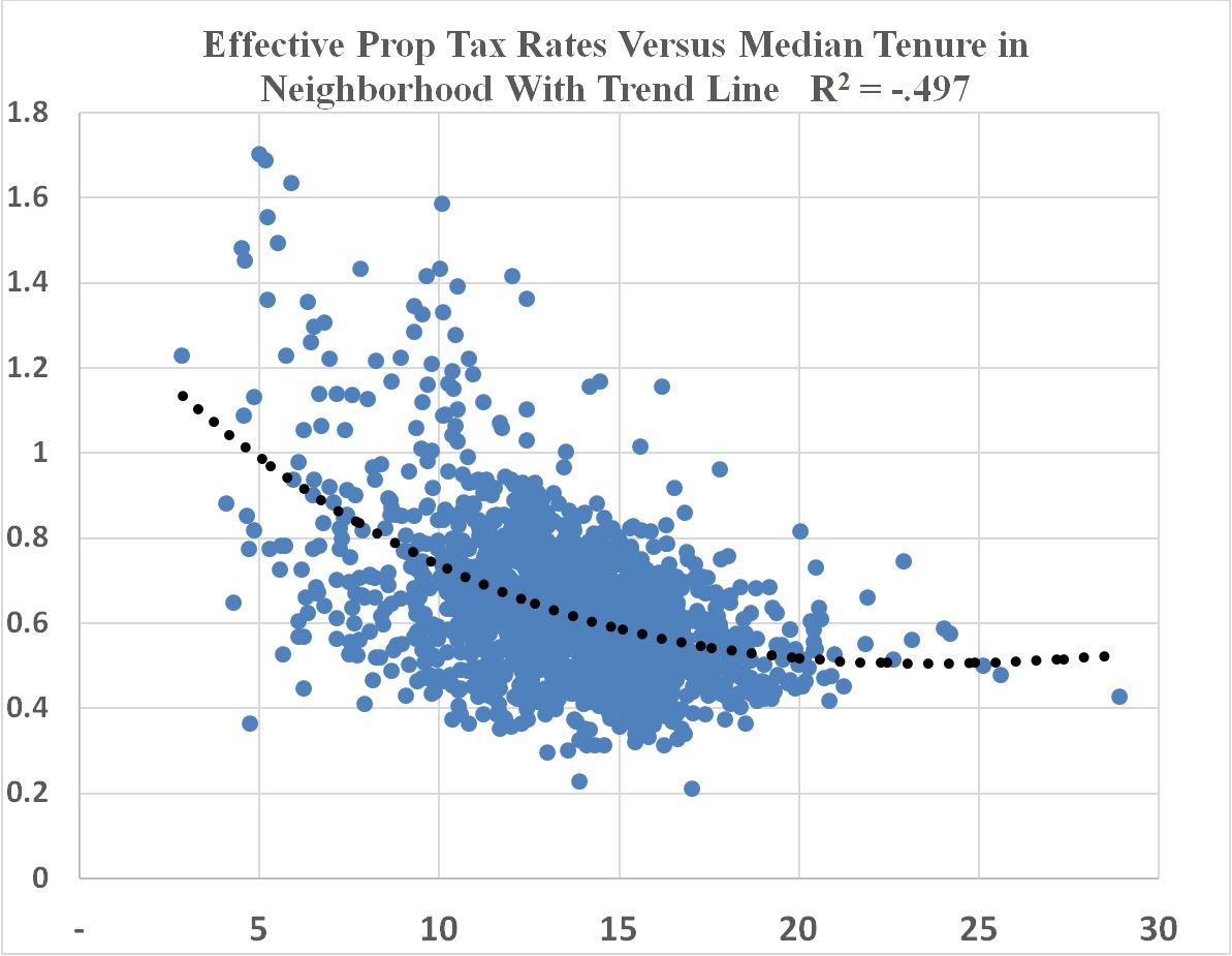
We observe the impact of Prop 13 on turnover in the neighborhoods within San Diego County, as shown in Exhibit 4 below. The correlation between the effective tax rate and average household tenure is a negative .497. The relationship appears non-linear so that as the effective property taxes drop below .60 the likelihood of staying put longer significantly increases.
Exhibit 4: The Impact of Lower Property Taxes on Household Tenure
A Preliminary Empirical Test on Price
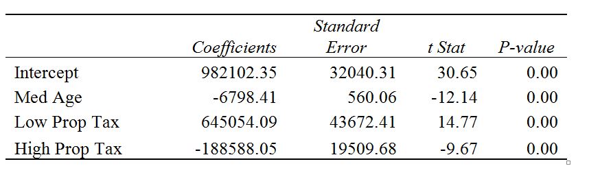
Looking at the general relationship between low and high tax paying neighborhoods and controlling for age with the average value as the dependent variable, we see the following regression results. Aside from age, the independent variables are low property tax rates (under.40%) and high (above .60%). While older homes sell for less in general, those with low property tax burdens observe a huge price premium compared to average or high property tax burden homes. Clearly there could be other variables that correlate with lower property taxes and so it is not valid to claim that the observed premium here is a result of low property taxes. But the sign is correct and the regression coefficient is highly significant. What is apparent is that Prop 13 is making some neighborhoods less affordable than others as prices are artificially held higher than in a market with more evenly distributed tax burdens.
Multiple R 0.44302
R Square 0.19627
Adjusted R Square 0.19479
Standard Error 337741
Observations (neighborhoods) 1632
Premiums of 10% to 20% as suggested by theoretical studies are not unreasonable based on these preliminary results. At the same time the present value to the owners of lower tax burden property are likely to average much higher percentages of property value as demonstrated next.
A Simulation of the Future Based on the Past
Imrohoroğlu, A., Matoba, K., & Tüzel, S. (2014) had suggested 17% increases in property values and K. Rosen (1982) had suggested about the same percentage. Here two simple measures of present value are applied to the housing price averages in San Diego County from 1979 through 2014 using actual averages and then simulated from 2015 through 2098, shown through 2067. The simulated prices were based on three assumptions, (1) average annual price increases of approximately 5.6% per year similar to the trend from 1979 through 2014, (2) a standard deviation of variation in annual appreciation of 8% similar to historical trends, and (3) serial correlation of .7 from year to year so as to incorporate the momentum of trends typically observed. Next the home price series are generated and property taxes are determined based on increasing a maximum of 2% from the prior year. Values are allowed to go down or up, but again the 2% max rule is imposed. Over time the difference between the actual property taxes paid and the market based full taxation are noted. Next a present value is calculated based on a 3% discount rate, which is far lower than Rosen might have used in 1982, but it is still higher than 30 year treasury bonds so one might argue it is too high for a certain return discount rate. This discount rate is applied to two different measures, one a fixed annuity based on the current difference in property taxes paid full assessment but discounted as a perpetuity, lasting forever. The other method employs perfect anticipation of future home prices and assumes the present value of the differences in property taxes paid over just 30 years. Not these methods are arbitrary but reasonable theories. The resulting present value of saved property taxes as a percentage of the value of the home are shown by year in Exhibit 5. The analysis is carried through 2098 but ends in 2067 since it is based on a perfect forward looking 30 years in the one case and the current year difference carried out permanently in the other case.
Exhibit 5: The Impact of Lower Property Taxes Discounted and Shown as a Percentage of the Current Home Value

What is quite astonishing in Exhibit 5 is the implication that the present value of the certain or anticipated property taxes can be, and will be, as much as 30% to 50% of the value of the home. One reason for this is the low discount rate; another is the long time horizon over which savings may accrue. But not only are these tax savings an enormous benefit they are also untaxed benefits. Unlike debt forgiveness which is usually treated as taxable income, property tax forgiveness is not taxed.
The Exhibit 5 is a personal value benefit to a current homeowner and should not be construed as the impact on the value of the home, but it does add greatly to the reservation prices that sellers which to obtain prior to moving and so again, market value premiums of 10% to 20% are highly reasonable in neighborhoods where a larger proportion of homes have low tax burdens. Whatever, the premium that exists now, it appears that this premium will continue to grow over time and the California housing market will wallow in a bog of its own creation with the ultimate in sticky supply added to an already supply constrained market.
Implications and Conclusions
Prop 13 disparities in property tax burdens are well known. What may not be as well-known is how the lower effective property tax rates over time reduces turnover rates. California already has well below normal turnover rates for existing housing compared to other states and this will only exacerbate over time. In the absence of Prop 13 people would move much more frequently, downsizing or upsizing and fixing up new homes. The revenues to the brokerage industry are at least a third less than normal as of 2014 as a result of Prop 13. The same can be said for moving companies and all the associated industries that benefit from the sale of housing, from appraisers to mortgage lenders to title companies to carpet sellers and painters and so forth.
Proponents of Prop 13 suggest that elderly will be pushed from their homes if California would ever repeal the law, and there is no politician willing to suggest changing the law, but it is really the grandsons and granddaughters who will be yelling the loudest for a maintenance of this law. Their untaxed benefits in present value terms will equal a third or more of the value of their home. Prop 13 will continue to spread the tax burden towards the newest of California’s home buyers, or require other forms of taxes, and subsidize those lucky enough to own a home in California bought closer to 1978 or during dips in home values.
For those states considering similar tax proposals to “protect” their elderly citizens, they should recognize that it does much more than just limit property tax increases. Housing turnover is reduced and home prices in affected neighborhoods may be artificially increased through a lack of supply.
References:
Imrohoroğlu, A., Matoba, K., & Tüzel, Ş. (2014). “Proposition 13: An Equilibrium Analysis” http://www.minneapolisfed.org/research/events/2014_05-14/Imrohoroglu_Prop13.pdf
Wasi, N., & White, M. J. “Property Tax Limitations and Mobility: Lock-in Effect of California’s Proposition 13”. http://econweb.ucsd.edu/~miwhite/wasi-white-final.pdf
Ferreira, Fernando V., “You Can Take It with You: Transferability of Proposition 13 Tax Benefits, Residential Mobility, and Willingness to Pay for Housing Amenities” (June 2004). UC Berkeley Center for Labor Economics Working Paper No. 72. http://dx.doi.org/10.2139/ssrn.661421
Rosen, Ken; The Impact of Proposition 13 on House Prices in Northern California: A Test of the
Interjurisdictional Capitalization Hypothesis,” Journal of Political Economy, 90:1 (1982),
191-200.
Stoks, Mark H. and Y.W. Park “ Residential Stability or Rational Bubble: Proposition 13 in Southern California”, International Real Estate Review, 2007, 10:1 pp 26-47
Tiebout, Charles, “A Pure Theory of Local Expenditures” The Journal of Political Economy, 64: 5, Oct. 1956, pp 416-424 A review is available at http://www.csiss.org/classics/content/43
Appendix: 1 Effective Property Tax Rates
Source: County of San Diego Office of Property Tax Services
Date: 9/29/2014
San Diego County Effective Property Tax Rate
City of Carlsbad 1.0710
City of Chula Vista 1.1185
City of Coronado 1.0478
City of Del Mar 1.0250
City of El Cajon 1.2142
City of Encinitas 1.0605
City of Escondido 1.1273
City of Imperial Beach 1.1662
City of La Mesa 1.1787
City of Lemon Grove 1.1909
City of National City 1.1030
City of Oceanside 1.0619
City of Poway 1.0949
City of San Diego 1.1790
City of San Marcos 1.0903
City of Santee 1.1644
City of Solana Beach 1.0250
City of Vista 1.0790